总结在R中使用corrplot绘制相关性图。
1. 加载数据
1 | # 加载数据,数据需转换成矩阵 |
2. 计算相关性系数
corrpolt用法:
1 | corrplot( |
1 | M <- cor(mtcars) |
3. 绘图
展示方式:
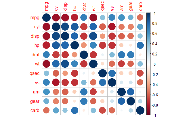
1 | corrplot(M) |
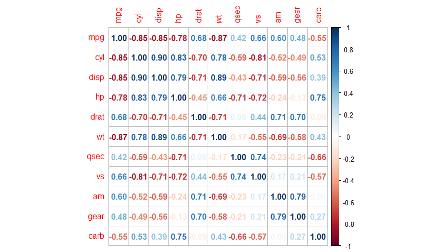
1 | corrplot(M,method="number") |
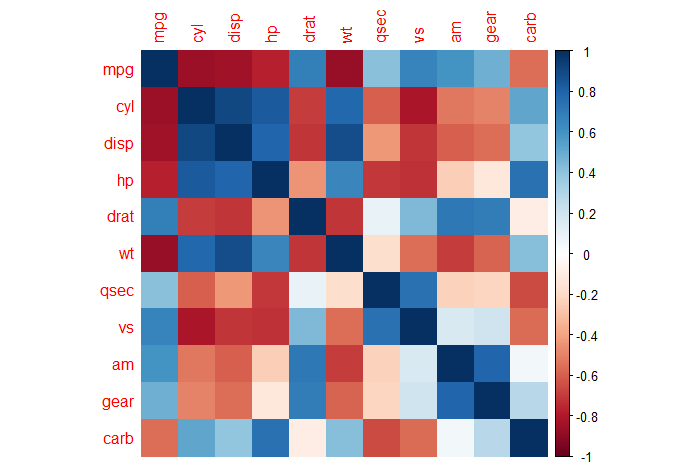
1 | corrplot(M,method="color") |
method还有其他选项:square、shade、pie、ellipse等。
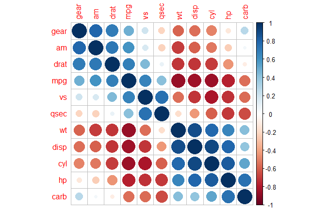
排序:
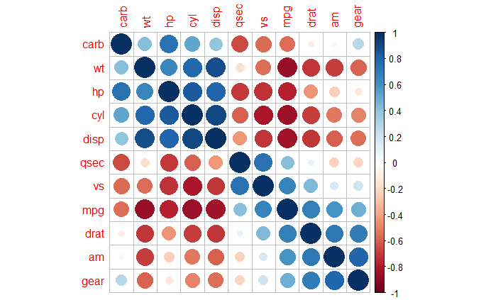
1 | corrplot(M,order = "hclust") |
1 | corrplot(M,order = "AOE") |
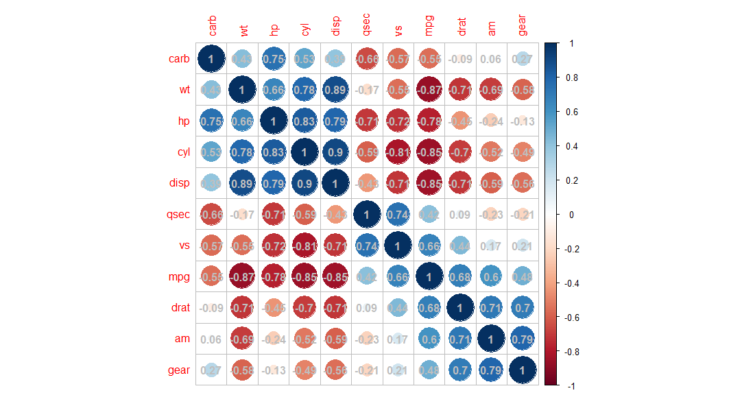
添加相关性系数数值:
1 | corrplot(M,order = "hclust",addCoef.col = "grey") |
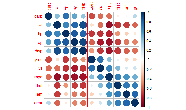
添加聚类框:
1 | corrplot(M, order = "hclust",addrect = 2,rect.col='red') |
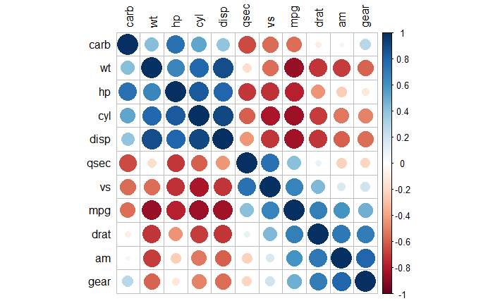
修改颜色:
1 | corrplot(M, order = "hclust",tl.col='black') |
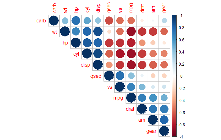
设置展示类型
type可以选upper、lower、full。
1 | corrplot(M, order = "hclust", type='upper') |
4. pvalue不显著的不显示
1 | # 先进行显著性检验 |
默认的会对不显著的打叉: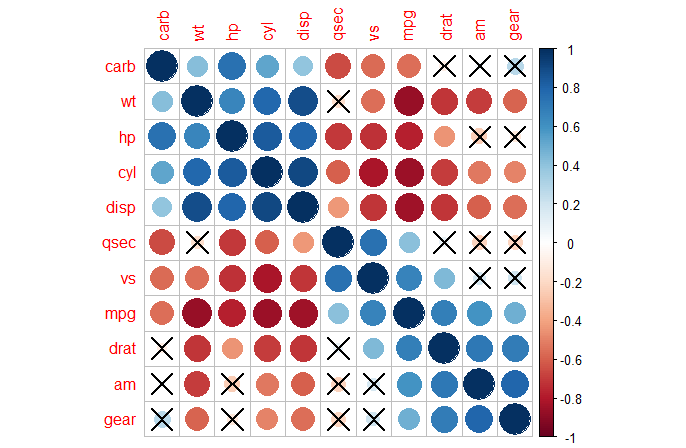
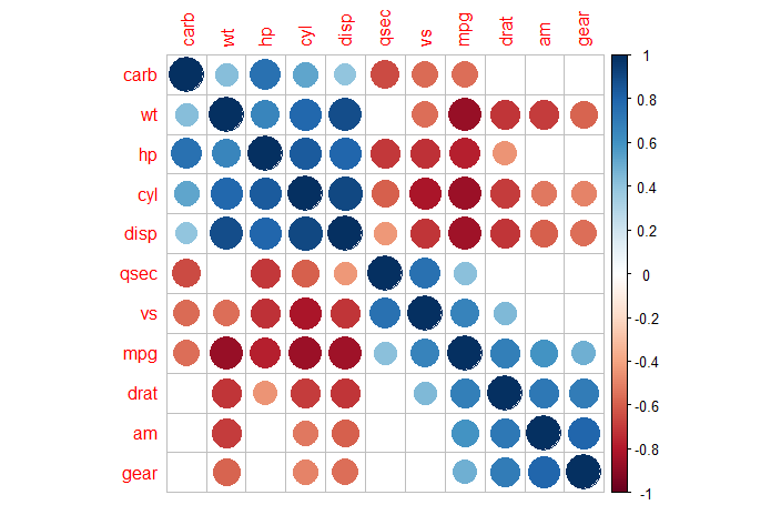
添加insig参数,指定不显著的为空
1 | corrplot(M, order = "hclust", p.mat = corrl$p,insig = "blank") |
显示pvalue的*。
1 | corrplot(M, order = "hclust", |

以上是corrplot主要功能。注意,corrplot包只适用于正方形,也就是说横向和纵向一样的去比较。